Writing Assignments

Each assignment applies one of the models that we studied in class to a real world question. The answer should be a document of 2-4 pages in length.

A good answer does not just apply the model mechanically to the problem. It also thinks about aspects that the model misses and modifies the answer accordingly.

Be sure to really explain your answer. In your graphs, explain which curves shift, by how much, and why. Explain the economic process that leads to the changes depicted in the graph.

How to submit

Please submit your submission via Gradescope any time prior to midnight of the due date.

Hand-written documents are fine, but make sure I can read them.

If you submit an image, please use scanning software. Do not submit photos (those are hard to read).

Assignment 1: IS/LM

Financial innovation has made money demand more interest elastic. Your task is to assess whether this change makes monetary and fiscal policy more or less effective.

Specifically, assume that the slope of the \(L(i)\) function gets steeper in the LM curve \(M/P = Y \times L(i)\). Determine the effects of a given change in \(M/P\) and \(G\) on equilibrium output for large and small slopes. Illustrate your answer in graphs (with explanations). Explain the economic intuition for what you find.

Be careful about how much the curves shift due to the shock. This may change with the slope parameter. It may help to assume a linear money demand function, so that LM becomes \(M/P=Y + L_0 - b_L \times i\).

For this question, I want you stay "inside the model." The IS/LM assumption of fixed prices is an obvious limitation, but we will live with it for now. There is no need to discuss what the model misses for this case.

Answer sketch

Assignment 2: AS/AD

The Fed has invested a great deal of effort in order to "anchor" inflation expectations at its target of two percent per year.

Here, we try to get a sense of why this makes sense through the lens of the AS/AD model. Since that model does not have inflation yet, we assume instead that the Fed can anchor expectations about price levels \(P^e\).

Suppose the economy is hit by a temporary negative supply shock. The shocks shifts \(m\) up, thereby lowering SR-AS and MR-AS. However, after some time \(m\) returns to its original value (and SR-AS and MR-AS shift back to their original positions).

Consider the implications for output and prices over time for the following scenarios:

1. The Fed does nothing. Price expectations adjust as usual. How would output and prices evolve over time? Explain the intuition.
2. Now consider the case where price expectations are well anchored (treat them as fixed). How does this change the outcome? What does the Fed gain from anchoring expectations. Hint: What happens to SR-AS while \(m\) is high?
3. Next consider the case where the Fed stabilizes output at the original (pre shock) \(Y_n\) through the entire episode. Price expectations move around as usual. Is there a risk that inflation expectations might get entrenched (although that is not in our model)?
4. Finally, consider the case where the Fed stabilizes output but price expectations are well anchored. Are the outcomes better than with price expectations that move around?

Be sure to explain the economic intuition for everything that happens.

It is likely easiest to do case 2 before case 1 and to do case 4 before case 3.

Assignment 3: Open Economy

This assignment considers how monetary policy effects spill over across borders.

Specifically, consider the implications of tighter foreign monetary policy (higher \(i^*\)) on the domestic economy. Assume floating exchange rates.

1. Explain how a higher \(i^*\) shifts the domestic AD curve. What is the mechanism?
2. Explain what happens to the domestic economy in the medium run \((Y, P, i, C, I,E, NX)\). Show that \(i < i^*\), even though \(i \uparrow\). Be sure to explain the sequence of events that lead to the changes in economic terms.
3. Explain what happens in the short run to the same variables. Again, explain the sequence of events.
4. Now suppose that the Fed tries to avoid the crowding out that occurs in the medium run (the drop in \(I\)). What would the Fed have to do to stabilize medium run investment? What happens to the same variables in that case?
5. The MR outcomes implies that \(i < i^*\). What would have to happen to \(E\) over time (after the medium run equilibrium is reached) to satisfy UIP? What does this finding suggest about the sustainability of an outcome where \(i \ne i^*\)?
6. Finally consider the case where the Fed tries to stabilize the dollar instead. What would the Fed have to do to keep the exchange rate stable? What are the implications for the domestic economy in that case?

Answer sketch

Example

Suppose that the interest elasticity of investment rises. Does this make monetary and fiscal policy more or less effective?

Since we are working in an IS/LM framework, we start with the model equations:

1. IS: \(Y=\bar{Z} + (b_1 + c_1)Y - b_2 i\)
2. LM: \(M/P = Y \times L(i)\)

We are considering how a higher \(b_2\) changes the effects of a given change in \(G\) or \(M\).

How does a higher \(b_2\) change the graph?

Let's write IS as \(i = \frac{\bar{Z} - (1 - b_1 - c_1) Y}{b_2}\). A higher \(b_2\) makes the IS curve flatter. The intuition is as follows. Starting from a point on IS, suppose we raise \(Y\). That moves us to the right of the IS curve where we have excess supply of goods (a unit increase in \(Y\) only leads to an increase in demand of \([1-b_1-c_1]\)). A lower \(i\) is required for goods market clearing. If \(b_2\) is high, a small drop in \(i\) leads to a large increase in \(I\) and is sufficient to restore market clearing. Therefore, IS is flat.

The value of \(b_2\) also affects the intercept of IS, but we do not care about that right now.

Fiscal shock

Increasing government spending by \(\Delta G\) shifts IS to the right by \(\frac{\Delta G}{1 - b_1 - c_1}\), which is independent of \(b_2\). Note: if we considered the vertical shift, \(\Delta G / b_2\), it would depend on \(b_2\) which makes life harder.

We may now compare the effects of a given change in \(G\) for high and low elasticities \(b_2\). To do so, we draw an IS/LM diagram with one LM curve and two IS curves that intersect LM in the same point (for easy visualization).

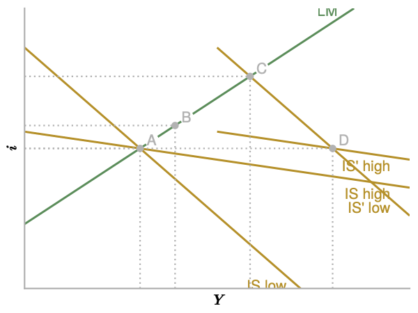
The economy starts at point A in both cases. The IS curves shift right by a given amount, so they intersect at point D. The new equilibria are given by B (high elasticity) and C (low elasticity). In the high elasticity (flat IS) case, output rises less.

Now we turn to the intuition. Starting at A, higher \(G\) raises demand and therefore output to point D (in both cases). At D we have excess demand for money. Households sell bonds, which drives up the interest rate. Higher interest rates crowd out investment and output starts to fall.

If investment responds strongly to interest rates, this crowding out effect is strong. A given increase in \(i\) causes a large decline in demand and therefore \(Y\). This is why the equilibrium increase in \(Y\) is small when investment is interest sensitive.

So the basic intuition is really very simple (but hard to see clearly without the model): A shock to aggregate demand causes interest rates to rise. Crowding out dampens the increase in output. If demand is interest sensitive, crowding out is strong.

Monetary shock

A similar write-up would go here...

---